Injection / Particle Generation

This module introduces the Injection command in PASS, which is used to generate specific particle distributions at the simulation starting position and inject the beam. The injection command supports independently setting transverse distribution, longitudinal distribution, beam parameters, offsets, etc. for each bunch, and is the entry point for particle simulation.

This example demonstrates how to construct specific particle distributions. The input files and running code used in this document can be found in GitHub example code .

Code location

Source file: PASS/commands/injection.py
Class name: Injection (inherited from Command )
Registration name: injection
Auxiliary class: InjectionBunchInfo (same file, responsible for parameter parsing and distribution generation of a single bunch)

Interface parameters

The parameters of the Injection command are shown in the table below. Here s must be 0 (the injection point is fixed at the starting position of the sequence), name is automatically filled by the sequence key name, and bunch0 , bunch1 , … are the parameter dictionaries of each bunch.

Property	JSON key	Type	Unit	Description
`s`	`S (m)`	float	m	Injection position (must be 0)
`name`	`name`	str		Element name, automatically filled by the sequence key name
`harmonic_number`	`Harmonic Number`	int		Bunch-grouping count; declare the same number of `bunch0`, `bunch1`, … dictionaries and use empty bunches for unfilled groups
`random_seed`	`Random Seed`	int or null		Optional seed for particle-distribution generation. Omit it, or set it to `null`, for a non-deterministic seed; a supplied value, including 0, makes the generated distribution reproducible for the same input and execution order
`bunch0`	`bunch0`	dict		Parameter dictionary of the 0th bunch
`bunch1`	`bunch1`	dict		Parameter dictionary of the 1st bunch
…	…	dict		Parameter dictionaries of more bunches

Bunch parameters

Each bunch uses bunch0 , bunch1 , … as keys, and the value is a dictionary containing all parameters of that bunch. The parameters are described below in five groups: transverse, longitudinal, beam, distribution, and offset.

Transverse parameters

Property	JSON key	Type	Unit	Description
`alphax`	`Alpha x`	float		Horizontal Twiss parameter \(\alpha_x\)
`alphay`	`Alpha y`	float		Vertical Twiss parameter \(\alpha_y\)
`betax`	`Beta x (m)`	float	m	Horizontal Twiss parameter \(\beta_x\)
`betay`	`Beta y (m)`	float	m	Vertical Twiss parameter \(\beta_y\)
`emitx`	`Emittance x (m'rad)`	float	m·rad	Horizontal emittance \(\varepsilon_x\)
`emity`	`Emittance y (m'rad)`	float	m·rad	Vertical emittance \(\varepsilon_y\)
`dx`	`Dx (m)`	float	m	Horizontal dispersion function \(D_x\)
`dpx`	`Dpx`	float		Horizontal dispersion derivative \(D_{px}\)
`dist_trans`	`Transverse dist`	str		Transverse distribution type, options: `gaussian` , `kv` , `waterbag` , `parabolic` , `uniform`

Longitudinal parameters

Property	JSON key	Type	Unit	Description
`sigmaz`	`Sigma z (m)`	float	m	Longitudinal bunch length RMS value \(\sigma_z\)
`dp`	`Sigma dp/p`	float		Momentum spread RMS value \(\sigma_{\delta}\)
`dist_longi`	`Longitudinal dist`	str		Longitudinal distribution type, options: `gaussian` , `coasting` , `matchz` , `matchdp`
`rf_voltage`	`RF Voltage (V)`	float	V	RF voltage (required for `matchz` and `matchdp` distributions)
`rf_phi`	`RF Phase (rad)`	float	rad	RF phase \(\phi_s\) (required for `matchz` and `matchdp` distributions)
`harmonic_num`	Injection-level `Harmonic Number`	int		Bunch-grouping count \(h_{\mathrm{group}}\) passed down from the Injection level. It is also used by `matchz` / `matchdp` to set the longitudinal scale, but does not constrain the RFCavity harmonic
`harmonic_id`	`Harmonic ID of this bunch`	int		Bunch-group index \(h_{\mathrm{id}}\), defining the fixed center \(z_{\mathrm{center}}=h_{\mathrm{id}}C/h_{\mathrm{group}}\)
`rf_position`	`RF S Position Refer to Inj. Point (m)`	float	m	Longitudinal position of the RF cavity relative to the injection point, used to back-propagate the distribution generated at s_rf to the injection point s=0
`ddp`	`Momentum Offset dp`	float		Bunch-level average momentum deviation \(\delta_0\) , added to each particle’s dp. Mutually exclusive with `dde`
`dde`	`Kinetic Energy Offset (eV)`	float	eV	Bunch-level kinetic energy offset, internally converted to `ddp` . Mutually exclusive with `ddp`

Beam parameters

Property	JSON key	Type	Unit	Description
`Ek`	`Kinetic Energy per Nucleon (eV/u)`	float	eV/u	Kinetic energy per nucleon
	`Number of Real Particles`	float		Number of real particles
	`Number of Macro Particles`	float		Number of macro particles
`stop_turn`	`Total Injection Turns`	int		Total injection turns
`interval`	`Injection Interval`	int		Injection interval (inject once every `interval` turns)

Distribution parameters

Property	JSON key	Type	Description
`is_load_dist`	`Is Load Distribution from File`	bool	Whether to load particle distribution from file
`load_dist_filepath`	`Distribution File Path`	str	Distribution file path ( `.tfs` format)
`is_save_init_dist`	`Is Save Initial Distribution`	bool	Whether to save the initial distribution
`insert_particles`	`Insert Particle Coordinate`	list	Insert specified particle coordinates, format is `[[x, px, y, py, z, dp], ...]`

Offset parameters

The horizontal offset ( Offset x ) and vertical offset ( Offset y ) have the same structure, each containing the following sub-parameters:

Property	JSON key	Type	Description
`is_offset`	`Is Offset`	bool	Whether to enable offset
`is_offset_fromfile`	`Is Load From File`	bool	Whether to load offset data from file
	`File Path`	str	Offset data file path ( `.tfs` format)
	`File Time Kind`	str	Time column type, options: `turn` , `time`
`offset_position`	`Offset Position (m)`	float	Position offset
`offset_momentum`	`Offset Momentum (rad)`	float	Momentum offset

Introduction to particle distribution types

In the PASS program, the initial particle distribution is implemented by the Injection command. In the Injection command, different distribution information can be set independently for each bunch.

Transverse particle distribution

Currently, the PASS program supports generating the following transverse particle distributions: horizontally-vertically decoupled 2D Gaussian distribution , 4D KV distribution , 4D waterbag distribution , 4D parabolic distribution , 2D uniform distribution in phase space .

The 4D distribution refers to defining a generalized hyper-ellipsoid boundary in the 4D phase space \((x, p_x, y, p_y)\). To simplify the derivation without loss of generality, we introduce normalized coordinates :

\[X = \frac{x}{a}, \quad P_x = \frac{p_x}{b}, \quad Y = \frac{y}{c}, \quad P_y = \frac{p_y}{d}\]

where \(a, b, c, d\) are the maximum physical envelope boundaries (hard boundaries) of the beam in the corresponding dimensions. Under this normalized coordinate system, the 4D hyper-ellipsoid boundary simplifies to a unit hypersphere:

\[r^2 = X^2 + P_x^2 + Y^2 + P_y^2 \le 1\]

The following describes each transverse particle distribution in detail. For 4D distributions, their projections onto the 1D plane have a unified power-law form. Let the distribution density in 4D phase space be \(f(r^2) \propto (1-r^2)^{\alpha}\) (alpha ge 0, defined within the 4D unit ball \(B^4\)), then the 1D marginal distribution for any single normalized coordinate \(u\) is:

\[\rho(u) \propto (1-u^2)^{\frac{n-1}{2}+\alpha}, \quad |u| \le 1\]

where \(n=4\) is the phase space dimension. For distributions uniformly distributed on the \(n\)-dimensional sphere \(S^{n-1}\) (such as KV), the 1D projection is:

\[\rho(u) \propto (1-u^2)^{\frac{n-3}{2}}\]

The 1D projections of each distribution are summarized below:

Distribution	4D density	\(\alpha\)	1D projection power	1D projection form
Uniform (2D square)	—	—	0	\(\rho(u) = \mathrm{const}\)
KV ( \(S^3\) sphere)	\(\delta(r-1)\)	—	\(\frac{1}{2}\)	\(\rho(u) \propto \sqrt{1-u^2}\)
Waterbag ( \(B^4\) uniform)	\(1\)	0	\(\frac{3}{2}\)	\(\rho(u) \propto (1-u^2)^{3/2}\)
Parabolic ( \(B^4\) , \(1-r^2\) )	\((1-r^2)^1\)	1	\(\frac{5}{2}\)	\(\rho(u) \propto (1-u^2)^{5/2}\)

The following describes each transverse particle distribution in detail:

Independent 2D Gaussian distribution (Gaussian)

In the \(x-p_x\) and \(y-p_y\) phase spaces, transverse coordinates following a Gaussian distribution are generated independently. The particle distribution in transverse phase space uses a \(4\sigma\) truncation, i.e., only particles satisfying:

\[|x| \le 4\sigma_x, \quad |y| \le 4\sigma_y\]

are retained.

For the 2D phase space Gaussian distribution ( \(x-p_x\) and \(y-p_y\) ), the particle inclusion ratios corresponding to different RMS emittances are as follows:

\(\epsilon/\epsilon_{\mathrm{rms}}\)

Truncation range

Retained ratio

1

\(1\sigma\)

39.346934029%

2

\(\sqrt{2}\sigma\)

63.212055883%

4

\(2\sigma\)

86.466471676%

6

\(\sqrt{6}\sigma\)

95.021293163%

9

\(3\sigma\)

98.889100346%

16

\(4\sigma\)

99.966453737%

Therefore, under the \(4\sigma\) truncation condition, the particle loss ratio is very low (approximately \(3.3\times10^{-4}\) ), and the Gaussian tail can be considered fully covered.

The specific truncation ratio can be calculated using the following function:
import numpy as np

def fraction_by_emittance(epsilon, epsilon_rms):
    fraction = 1 - np.exp(-epsilon / (2 * epsilon_rms))
    print(f"eps/eps_rms = {epsilon/epsilon_rms}, particle proportion = {fraction:.9%}")

for epsi in (1, 2, 4, 6, 8, 9, 16, 25, 36):
    fraction_by_emittance(epsilon=epsi, epsilon_rms=1)
4D KV (Kapchinskij-Vladimirskij) distribution

In the \(x-p_x-y-p_y\) four-dimensional phase space, a particle distribution uniformly distributed on the surface of a four-dimensional hyper-ellipsoid is generated, which is an idealized distribution existing only on the 4D spherical shell. Under this distribution, the space charge field produced by the particles is strictly linear within the bunch, enabling a rigorous analytical solution of the space charge problem.

After integrating out two dimensions, the projection of the KV distribution onto any 2D plane (such as the \(x-p_x\) plane) is a uniformly filled ellipse. After further integrating out one dimension, the projection of the KV distribution onto the 1D plane is a semi-ellipse (or semi-circle) distribution. The detailed derivation is as follows: the KV distribution is uniformly distributed on the 4D hypersphere \(S^3\) ( \(r^2 = 1\) ). To obtain the 1D marginal distribution of \(u_x\), the remaining three coordinates on \(S^3\) need to be integrated:

\[\rho(u_x) \propto (1-u_x^2)^{\frac{n-3}{2}} = (1-u_x^2)^{\frac{1}{2}}\]

i.e., the 1D projection power is \(\frac{1}{2}\) .

Note

According to the integration: in the \(x-p_x\) and \(y-p_y\) phase planes, the full emittance of the KV distribution is 4 times the RMS emittance.

i.e., all particles in the KV distribution are within the \(2\sigma\) truncation range. However, the program still retains particles satisfying:

\[|x| \le 4\sigma_x, \quad |y| \le 4\sigma_y\]

4D Waterbag distribution

In the \(x-p_x-y-p_y\) four-dimensional phase space, a particle distribution uniformly distributed inside the four-dimensional hyper-ellipsoid is generated.

After integrating out two dimensions, the projection of the waterbag distribution onto any 2D plane (such as the \(x-p_x\) plane) follows a parabolic distribution. After further integrating out one dimension, the projection of the waterbag distribution onto the 1D plane is a \(\frac{3}{2}\) -power parabolic distribution. The detailed derivation is as follows: the waterbag distribution is uniformly distributed inside the 4D hyper-ball \(B^4\) ( \(f(r^2) = 1\) , i.e., \(\alpha = 0\) ). To obtain the 1D marginal distribution of \(u_x\), the remaining three coordinates on \(B^4\) need to be integrated, and the remaining part is a 3D ball of radius \(\sqrt{1-u_x^2}\) :

\[\rho(u_x) \propto V_3\!\left(\sqrt{1-u_x^2}\right) \propto (1-u_x^2)^{\frac{3}{2}}\]

where \(V_3(R) \propto R^3\) is the 3D ball volume. i.e., the 1D projection power is \(\frac{3}{2}\) .

Note

According to the integration: in the \(x-p_x\) and \(y-p_y\) phase planes, the full emittance of the waterbag distribution is 6 times the RMS emittance.

i.e., all particles in the waterbag distribution are within the \(\sqrt{6}\sigma\) truncation range. However, the program still retains particles satisfying:

\[|x| \le 4\sigma_x, \quad |y| \le 4\sigma_y\]

4D Parabolic distribution

In the \(x-p_x-y-p_y\) four-dimensional phase space, a particle distribution with density decreasing parabolically from the center outward as r increases is generated. This distribution is more realistic than the waterbag distribution for beams in real accelerators that tend to be concentrated toward the center.

After integrating out two dimensions, the projection of the parabolic distribution onto any 2D plane (such as the \(x-p_x\) plane) follows a quadratic parabolic distribution. After further integrating out one dimension, the projection of the parabolic distribution onto the 1D plane is a \(\frac{5}{2}\) -power parabolic distribution. The detailed derivation is as follows: the 4D density of the parabolic distribution is \(f(r^2) \propto (1-r^2)^1\) ( \(\alpha = 1\) ). To obtain the 1D marginal distribution of \(u_x\):

\[\rho(u_x) \propto (1-u_x^2)^{\frac{n-1}{2}+\alpha} = (1-u_x^2)^{\frac{3}{2}+1} = (1-u_x^2)^{\frac{5}{2}}\]

i.e., the 1D projection power is \(\frac{5}{2}\) .

Note

According to the integration: in the \(x-p_x\) and \(y-p_y\) phase planes, the full emittance of the parabolic distribution is 8 times the RMS emittance.

i.e., all particles in the parabolic distribution are within the \(\sqrt{8}\sigma\) truncation range. However, the program still retains particles satisfying:

\[|x| \le 4\sigma_x, \quad |y| \le 4\sigma_y\]

Uniform distribution

In the \(x-p_x\) and \(y-p_y\) phase spaces, 2D uniform square distributions are generated independently. For each transverse plane, uniform sampling is performed within the square region \([-1, 1] \times [-1, 1]\) in normalized coordinates \((u, v)\) , and then mapped to physical coordinates through Twiss parameters. The RMS emittance of this distribution is strictly equal to the input parameter \(\varepsilon\) , the full emittance is 3 times the RMS emittance, and all particles are within the \(\sqrt{3}\sigma\) truncation range. This distribution can simulate the initial beam produced by an electron gun, etc.

After integrating out one dimension, the projection of the uniform distribution onto the 1D plane is a constant (uniform) distribution. Since \(u_x\) and \(v_x\) are independently and uniformly distributed on \([-1, 1]\) , after integrating over \(v_x\):

\[\rho(u_x) = \frac{1}{2} = \mathrm{const} \propto (1-u_x^2)^{0}\]

i.e., the 1D projection power is \(0\) .

Longitudinal particle distribution

Currently, the PASS program supports generating the following longitudinal particle distributions: 2D Gaussian distribution , coasting beam distribution , distribution matched to RF parameters - longitudinal bunch length RMS value , distribution matched to RF parameters - momentum spread RMS value :

2D Gaussian distribution (Gaussian)

In the \(z-p_z\) phase space, longitudinal coordinates following a Gaussian distribution are generated. The particle distribution in longitudinal phase space uses a \(4\sigma\) truncation, i.e., only particles satisfying:

\[|z| \le 4\sigma_z\]

are retained.

Coasting beam distribution (Coasting)

In the \(z-p_z\) phase space, longitudinal coordinates are generated where \(z\) follows a uniform distribution and \(p_z\) follows a Gaussian distribution. The particles are not truncated in the longitudinal phase space; the longitudinal position coordinate has a maximum of half the circumference and a minimum of negative half the circumference.

Distribution matched to RF parameters - longitudinal bunch length RMS value (MatchZ)

In the \(z-p_z\) phase space, longitudinal coordinates satisfying both the RF parameters and the longitudinal bunch length constraint ( \(\sigma_z\) ) are generated. The particle distribution in longitudinal phase space uses a \(2\sigma\) truncation, i.e., only particles satisfying:

\[|z| \le 2\sigma_z\]

are retained.

Distribution matched to RF parameters - momentum spread RMS value (MatchDp)

In the \(z-p_z\) phase space, longitudinal coordinates satisfying both the RF parameters and the momentum spread constraint ( \(\sigma_{\delta}\) ) are generated. The particle distribution in longitudinal phase space uses a \(2\sigma\) truncation, i.e., only particles satisfying:

\[|z| \le 2\sigma_z\]

are retained.

Multi-bunch Longitudinal Coordinates

PASS defines the particle-array coordinate z as \(z_{\mathrm{rel}}\), measured relative to the center of the owning bunch. The fixed laboratory center of each bunch is determined by its group index:

\[z_{\mathrm{center}} = h_{\mathrm{id}}\frac{C}{h_{\mathrm{group}}}, \qquad z_{\mathrm{lab}} = z_{\mathrm{rel}} + z_{\mathrm{center}}.\]

Injection no longer shifts bunch centers into the particle z array and uses no odd/even harmonic branches. The generated longitudinal distribution is stored directly as \(z_{\mathrm{rel}}\).

If the distribution parameters are defined at an RF cavity position \(s=s_{\mathrm{rf}}\), injection applies only the linear back-propagation

\[z_{\mathrm{rel}}(0) = z_{\mathrm{rel}}(s_{\mathrm{rf}}) + \eta s_{\mathrm{rf}}\delta, \qquad \eta = \frac{1}{\gamma_t^2}-\frac{1}{\gamma^2}.\]

Injection does not fold \(z_{\mathrm{rel}}\) around the ring. Elements that need an absolute arrival phase, such as RFCavity, construct \(z_{\mathrm{lab}}\) themselves.

Bunch filling scheme

Note

The bunch ID ( bunch_id ) is strictly numbered starting from 0 with a step of 1, determined by the key names bunch0 , bunch1 , … in the input file. The number of bunches is determined by the number of bunch keys in the input file.

harmonic_id values must be unique and cover \(0,1,\ldots,h_{\mathrm{group}}-1\) exactly. The number of declared bunches therefore equals Harmonic Number. An unfilled slot is represented by a declared bunch with zero macro particles.

Full filling: every group contains particles, with centers at \(0,C/h_{\mathrm{group}},\ldots,(h_{\mathrm{group}}-1)C/h_{\mathrm{group}}\)
Partial filling: retain the complete group-index set and assign zero macro particles to the unfilled slots

The figure below illustrates bunch grouping around a ring of circumference \(C\). The marked points are \(z_{\mathrm{center}}\), and group indices increase clockwise. The upper figure shows full filling for \(h_{\mathrm{group}}=4\); the lower figure shows partial filling for \(h_{\mathrm{group}}=5\), with groups 1, 3, and 4 represented by empty bunches:

Dispersion coupling

If the injection point has dispersion functions \(D_x\) and \(D_{px}\) , then after generating the transverse distribution, dispersion coupling is automatically applied:

\[x \leftarrow x + D_x \cdot \delta, \quad p_x \leftarrow p_x + D_{px} \cdot \delta\]

where \(\delta\) is the particle’s momentum deviation. This ensures that the particle distribution and the longitudinal momentum spread are physically self-consistent.

Momentum deviation

During injection, an average momentum offset \(\delta_0\) can be applied to the entire bunch. When the particle distribution is generated, \(\delta\) follows a distribution with mean 0 (such as a Gaussian distribution \(\delta \sim \mathcal{N}(0, \sigma_\delta)\) ). After applying the offset, it becomes \(\delta \sim \mathcal{N}(\delta_0, \sigma_\delta)\) , i.e., the distribution center shifts from 0 to \(\delta_0\) . \(\delta_0\) is an additive quantity, not the total \(\delta\) of the particle. This is used to simulate scenarios such as injection energy offset and reference momentum offset.

Two input methods are supported (mutually exclusive; if both are non-zero, an error is raised):

Momentum deviation ( Momentum Offset dp ): directly provides \(\delta_0\) (dimensionless, relative to the reference momentum deviation)

Kinetic energy offset ( Kinetic Energy Offset (eV) ): provides \(\Delta E\) (in eV), internally converted to \(\delta_0\)

Exact conversion formula

The conversion from kinetic energy offset \(\Delta E\) to momentum deviation \(\delta_0\) uses the exact relativistic energy-momentum relation:

\[E^2 = p^2 + m_0^2\]

where \(E\) is the total energy ( \(E = E_k + m_0\) ), \(p\) is the momentum, and \(m_0\) is the rest mass. The parameters of the reference particle (no deviation) are:

\[E_0 = E_k + m_0, \quad p_0 = \sqrt{E_0^2 - m_0^2}\]

After applying the kinetic energy offset \(\Delta E\) , the particle’s total energy becomes \(E_1 = E_0 + \Delta E\) , and the corresponding momentum is:

\[p_1 = \sqrt{E_1^2 - m_0^2} = \sqrt{(E_0 + \Delta E)^2 - m_0^2}\]

Therefore, the momentum deviation is:

\[\delta_0 = \frac{p_1}{p_0} - 1 = \frac{\sqrt{(E_0 + \Delta E)^2 - m_0^2}}{\sqrt{E_0^2 - m_0^2}} - 1\]

This formula is fully exact , with no approximations, and is consistent with the exact \(E^2 = p^2 + m_0^2\) transformation used in the RF cavity.

First-order linearization approximation

For the formula \(\delta_0 = p_1/p_0 - 1\) , a first-order Taylor expansion is performed at \(\Delta E \to 0\) . From \(E \, dE = p \, dp\) we get:

\[dE = \frac{p}{E} \, dp = \beta \, dp \quad \Longrightarrow \quad dp = \frac{dE}{\beta}\]

where \(\beta = p_0 c / E_0\) is the reference particle velocity. Since in PASS \(\delta = \Delta p / p_0\) is the relative momentum deviation, the reference momentum \(p_0 = \beta \gamma m_0 = \beta E_0\) , therefore:

\[\delta_0 \approx \frac{\Delta E}{\beta^2 \, E_0}\]

This approximation truncates \(O(\delta_0^2)\) and higher-order terms. It has sufficient accuracy for small deviations, but significant errors for large deviations.

Comparison of exact and approximate formulas

The following table uses a proton ( \(E_k = 45\) MeV , \(\beta = 0.299\) ) as an example to show the differences between the two formulas at different \(\Delta E\) values:

\(\Delta E\) (eV)	Exact \(\delta_0\)	Approximate \(\delta_0\)	Relative error
1,000	1.137126e-5	1.137132e-5	0.000005%
10,000	1.137073e-4	1.137132e-4	0.000052%
100,000	1.136544e-3	1.137132e-3	0.000517%
1,000,000	1.131311e-2	1.137132e-2	0.0514%
10,000,000	1.084146e-1	1.137132e-1	4.89%
50,000,000	4.717485e-1	5.685659e-1	20.5%

For small deviations ( \(\Delta E < 100\) keV ), the two formulas have almost no difference, but for large deviations (e.g., \(\Delta E > 1\) MeV ), the linear approximation error exceeds 0.05%, and at \(\Delta E = 50\) MeV the error reaches 20%. PASS uses the exact formula to cover large deviation scenarios.

Application order

The momentum deviation \(\delta_0\) is applied to each particle’s \(\delta\) before the longitudinal offset:

\[\delta \leftarrow \delta + \delta_0\]

Therefore, the subsequent rf_position back-propagation ( \(z \leftarrow z + \eta \, s_{\text{rf}} \, \delta\) ) and dispersion coupling ( \(x \leftarrow x + D_x \, \delta\) ) both use the \(\delta\) value that includes \(\delta_0\) , ensuring physical self-consistency.

Input file

{
    "Beam Name": "proton",
    "Number of Protons": 1,
    "Number of Neutrons": 0,
    "Number of Charges": 1,
    "Transition Gamma": 4.8,
    "Number of turns": 5,
    "Circumference (m)": 251.327,
    "Backend (gpu/cpu)":"cpu",
    "Number of GPU devices": 1,
    "Device Id": [
        0
    ],
    "Output directory": "./output",
    "Is plot figure": true,
    "Sequence": {
        "Injection": {
            "S (m)": 0.0,
            "Command": "Injection",
            "Harmonic Number": 1,
            "bunch0": {
                "Kinetic Energy per Nucleon (eV/u)": 45e6,
                "Number of Real Particles": 100000000000.0,
                "Number of Macro Particles": 100000.0,
                "Is Load Distribution from File": false,
                "Distribution File Path": "",
                "Total Injection Turns": 1,
                "Injection Interval": 1,
                "Alpha x": -2.614303952,
                "Alpha y": 1.57442348,
                "Beta x (m)": 0.5,
                "Beta y (m)": 0.5,
                "Emittance x (m'rad)": 0.00019999999999999998,
                "Emittance y (m'rad)": 9.999999999999999e-05,
                "Dx (m)": 0.0,
                "Dpx": 0.0,
                "Sigma z (m)": 30,
                "Sigma dp/p": 0.005,
                "Transverse dist": "gaussian",
                "Longitudinal dist": "matchz",
                "RF Voltage (V)": 100e3,
                "RF Phase (rad)": 0.5235987755982988,
                "Harmonic ID of this bunch": 0,
                "RF S Position Refer to Inj. Point (m)": 0.0,
                "Offset x": {
                    "Is Offset": false,
                    "Is Load From File": false,
                    "File Path": "",
                    "File Time Kind": "turn",
                    "Offset Position (m)": 0.0,
                    "Offset Momentum (rad)": 0.0
                },
                "Offset y": {
                    "Is Offset": false,
                    "Is Load From File": false,
                    "File Path": "",
                    "File Time Kind": "turn",
                    "Offset Position (m)": 0.0,
                    "Offset Momentum (rad)": 0.0
                },
                "Is Save Initial Distribution": true,
                "Insert Particle Coordinate": [[0,0,0,0,0,0]]
            }
        },
        "StatMonitor1":{
            "S (m)": 0.0,
            "Command": "StatMonitor"
        }
    }
}

Run command

cd PASS\example\01_generate_distribution
python run.py --beam0=./beam0.json

Based on the input file above, a bunch with a Gaussian distribution in the transverse direction and a MatchZ distribution in the longitudinal direction will be generated. By modifying the following two parameter lines, the type of generated bunch distribution can be adjusted:

"Transverse dist": "gaussian",
"Longitudinal dist": "matchz",

The values for the transverse distribution are: gaussian , kv , waterbag , parabolic , uniform , and the values for the longitudinal distribution are: gaussian , coasting , matchz , matchdp .

When generating longitudinal gaussian and coasting distributions, RF-related parameters are not required. When generating matchz and matchdp distributions, RF parameters must be provided.

1D projection theoretical curves

The figure below shows the theoretical projection curves of the four transverse distributions ( Uniform , KV , Waterbag , Parabolic ) on the 1D plane. All curves are normalized to \(\int_{-1}^{1} \rho(u) \, du = 1\) , with the horizontal axis being the normalized coordinate \(u \in [-1, 1]\) . The increasing power trend from Uniform (flat-top) to Parabolic (peaked) can be clearly seen.

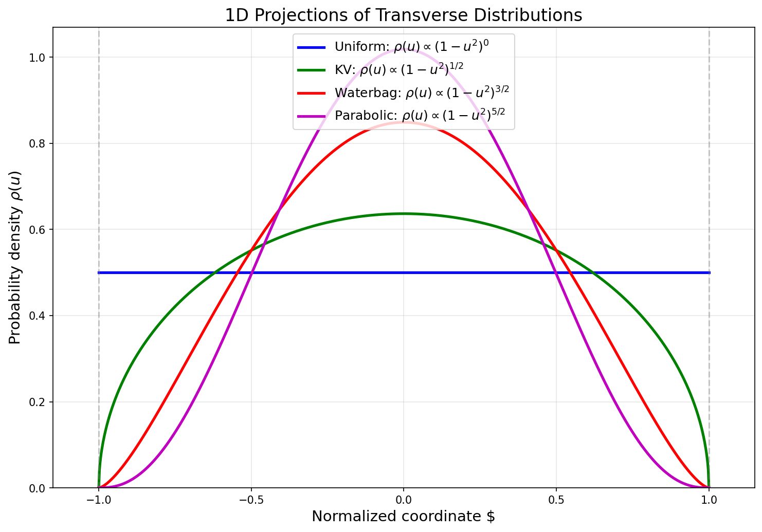
Figure 1. 1D projections of transverse distributions (theory)

Simulation results

Below, we show the simulated particle distribution figures obtained by keeping the Twiss, emittance, RF, and other parameters in the above input file unchanged and only changing the distribution type.

Transverse Gaussian distribution:

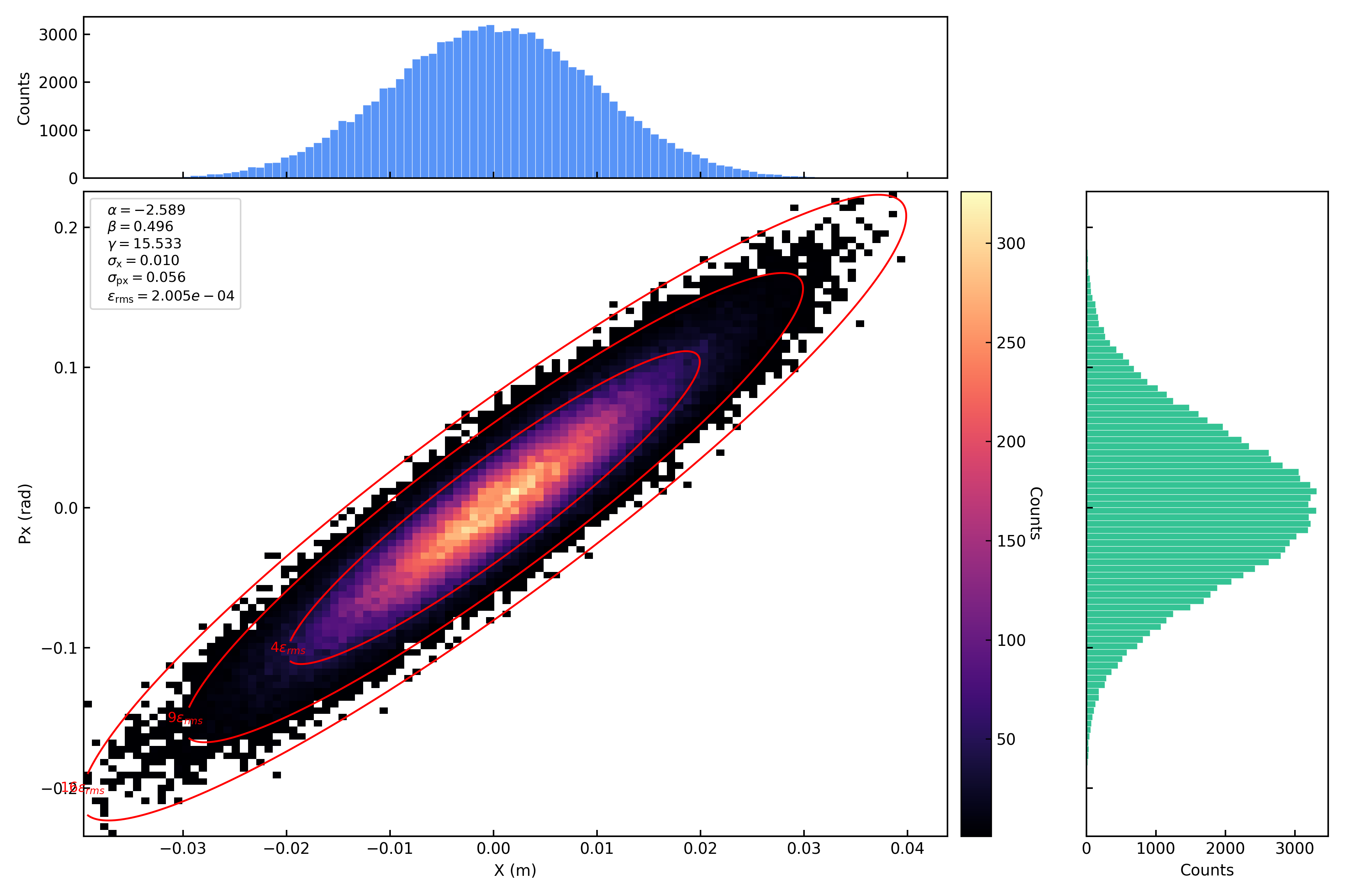
Gaussian x-px — Figure 2. Transverse gaussian distribution: x-px

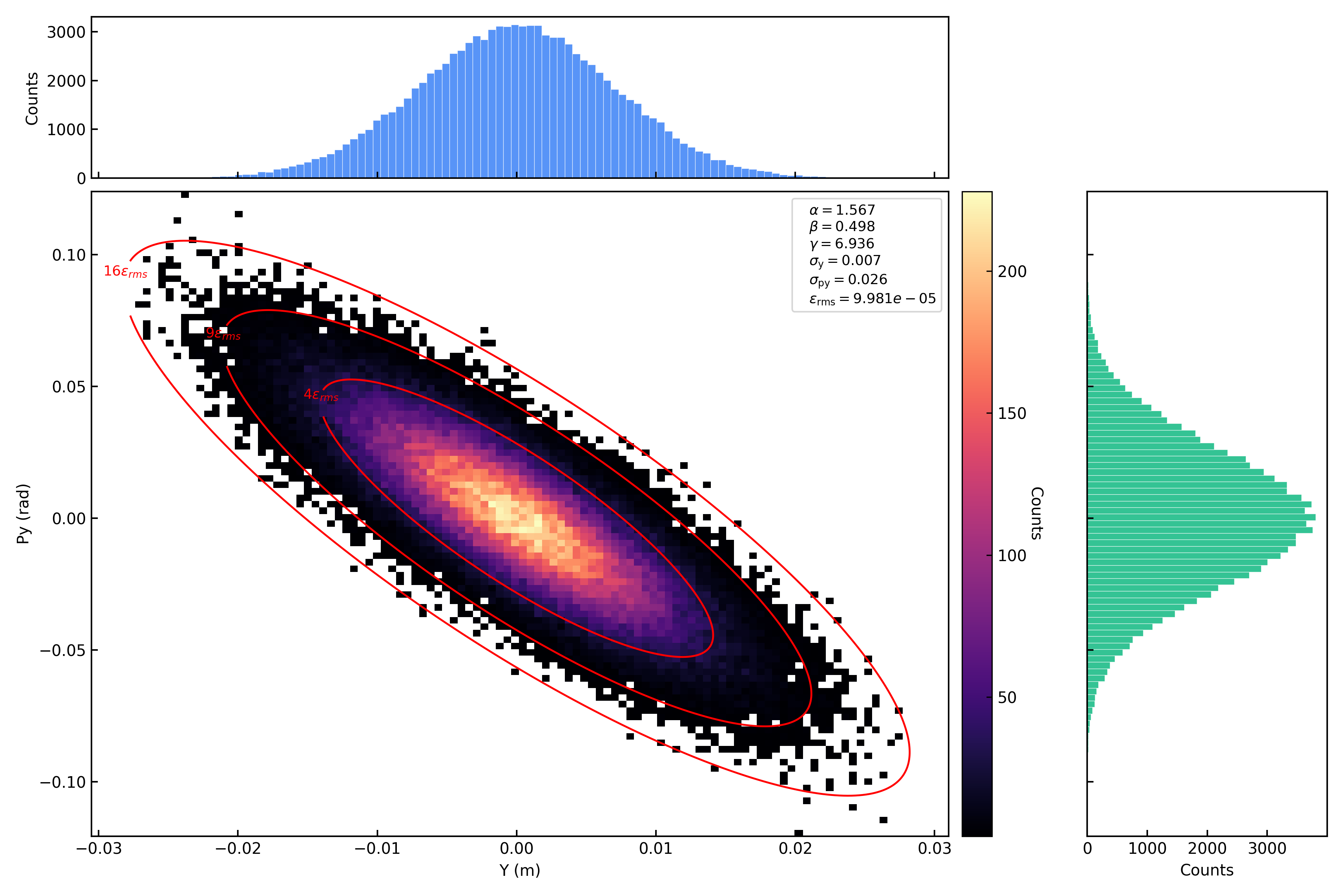
Gaussian y-py — Figure 3. Transverse gaussian distribution: y-py

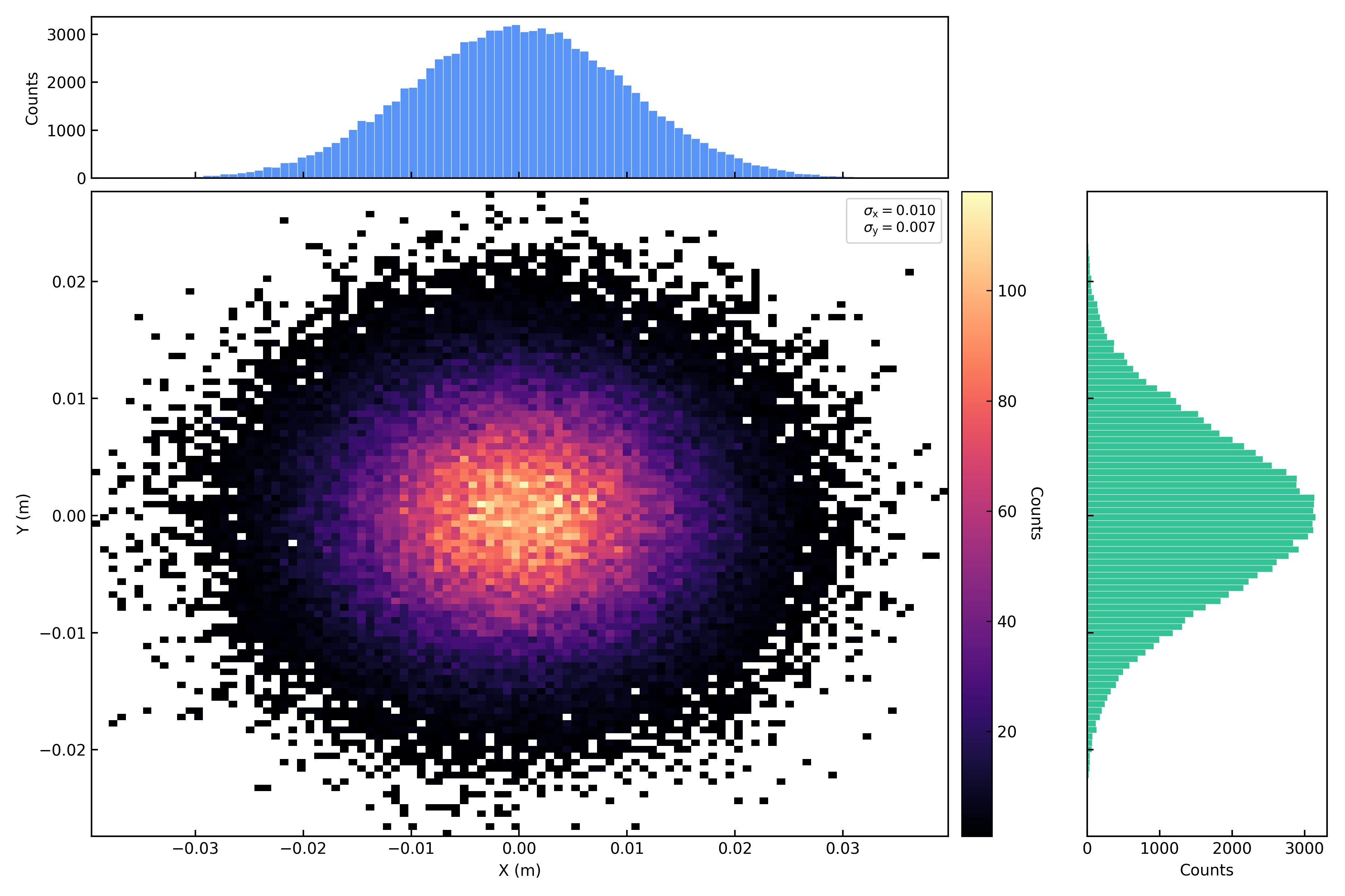
Gaussian x-y — Figure 4. Transverse gaussian distribution: x-y

Transverse KV distribution:

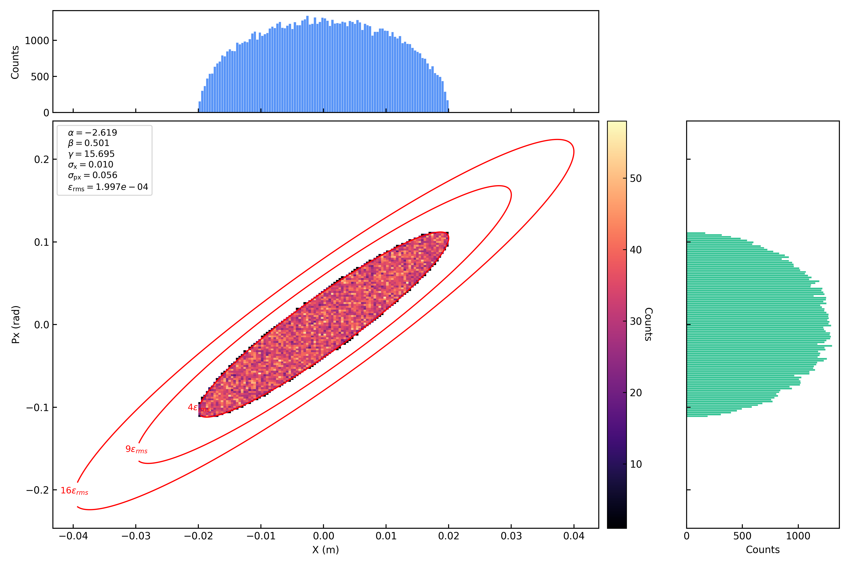
kv x-px — Figure 5. Transverse KV distribution: x-px

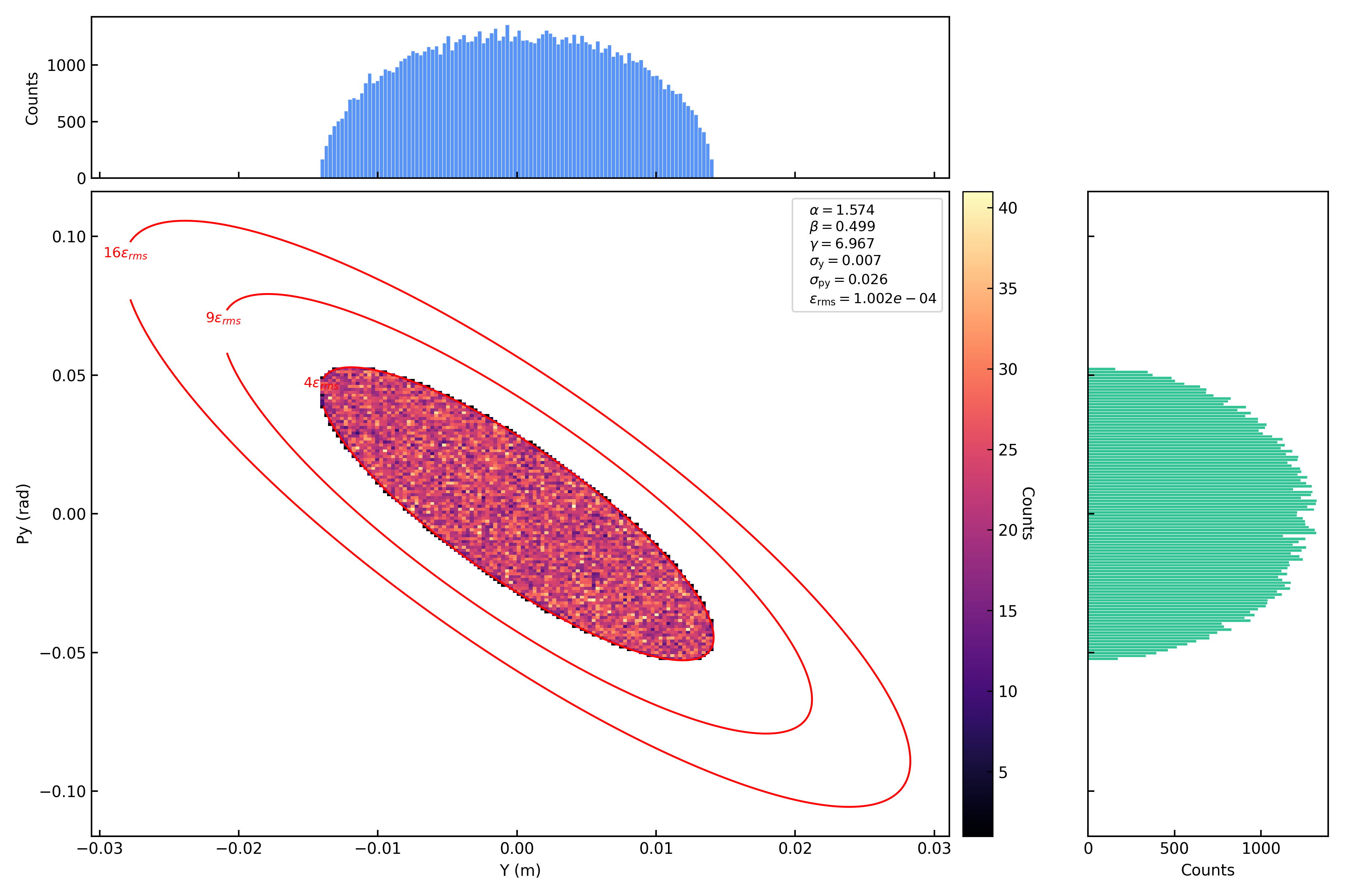
kv y-py — Figure 6. Transverse KV distribution: y-py

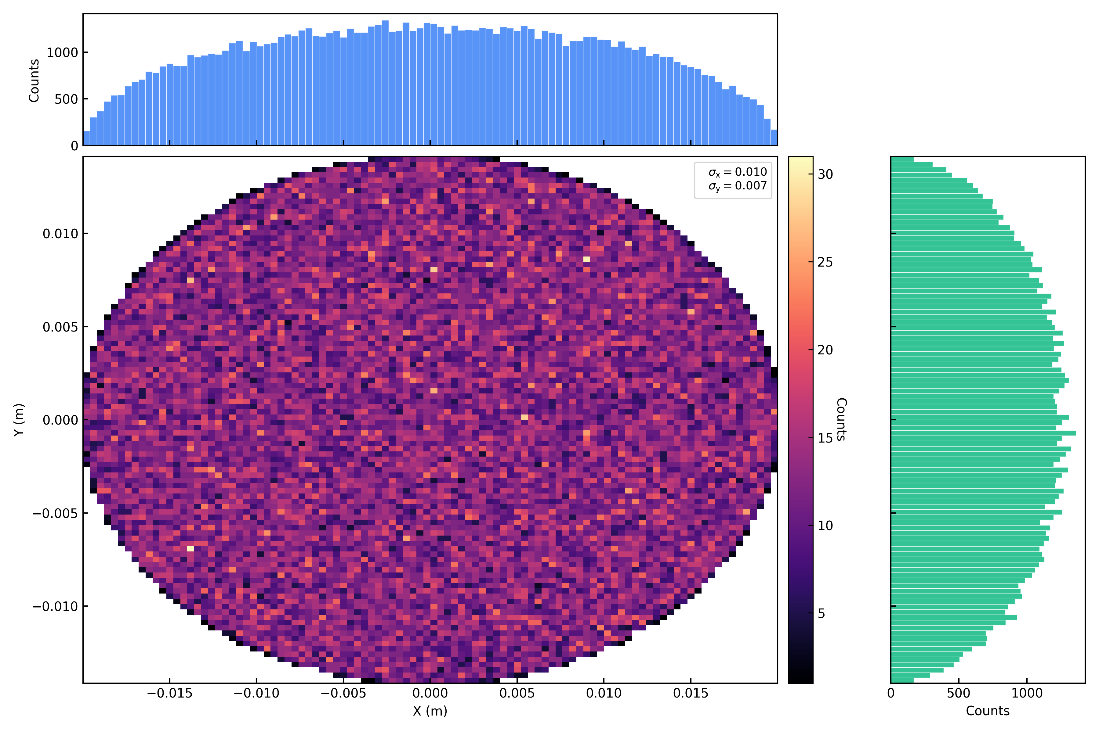
kv x-y — Figure 7. Transverse KV distribution: x-y

Transverse waterbag distribution:

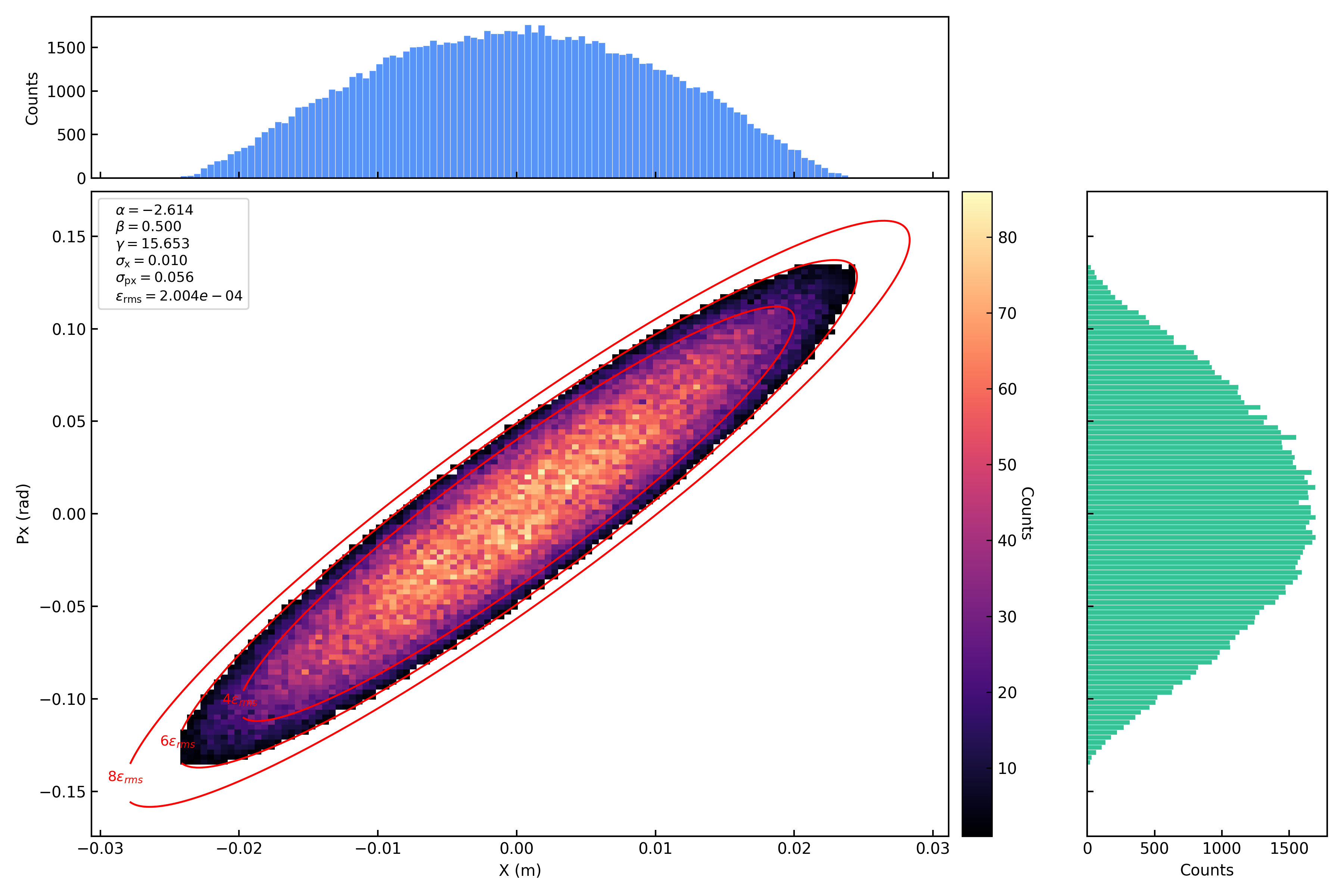
waterbag x-px — Figure 8. Transverse waterbag distribution: x-px

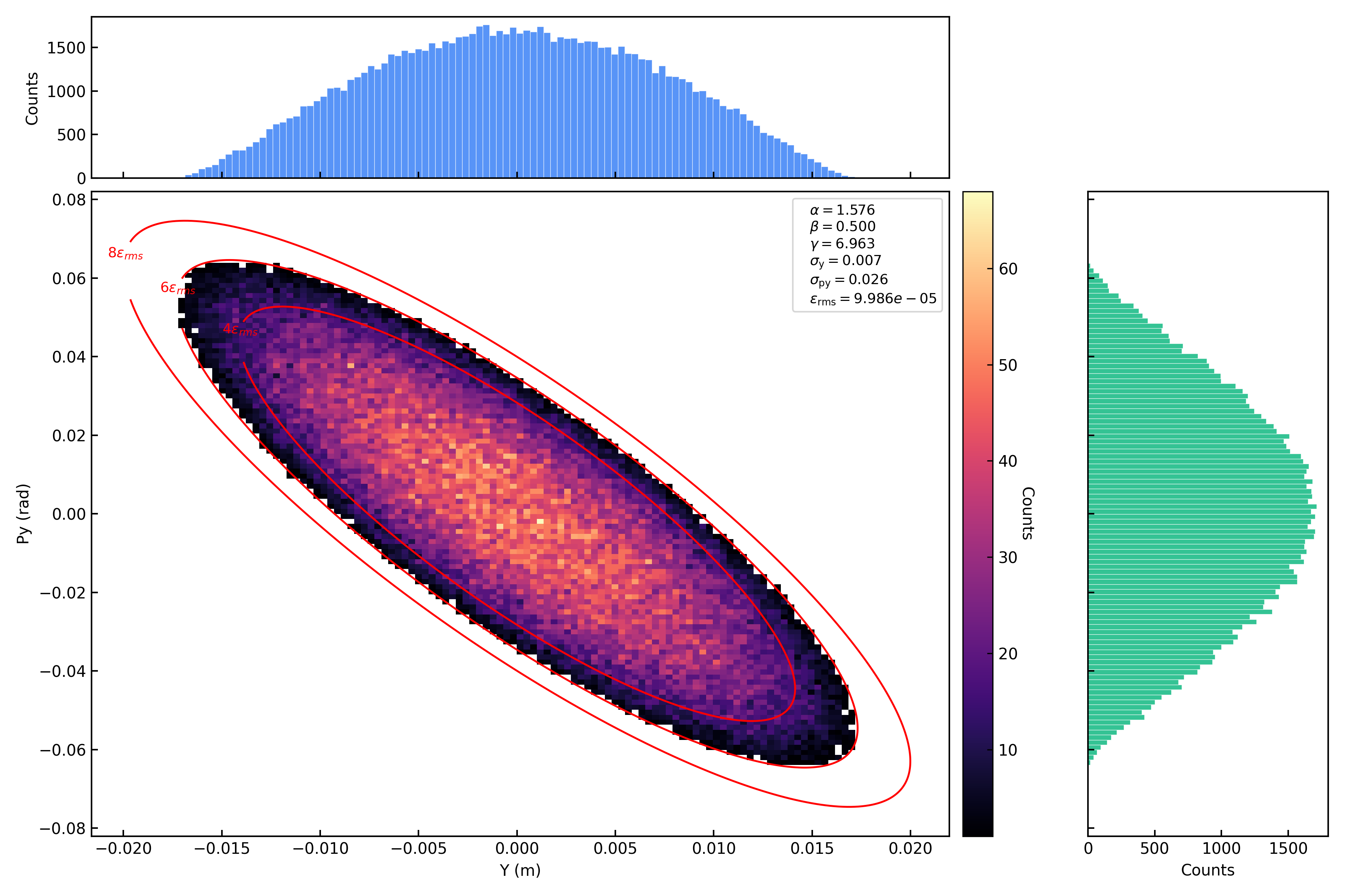
waterbag y-py — Figure 9. Transverse waterbag distribution: y-py

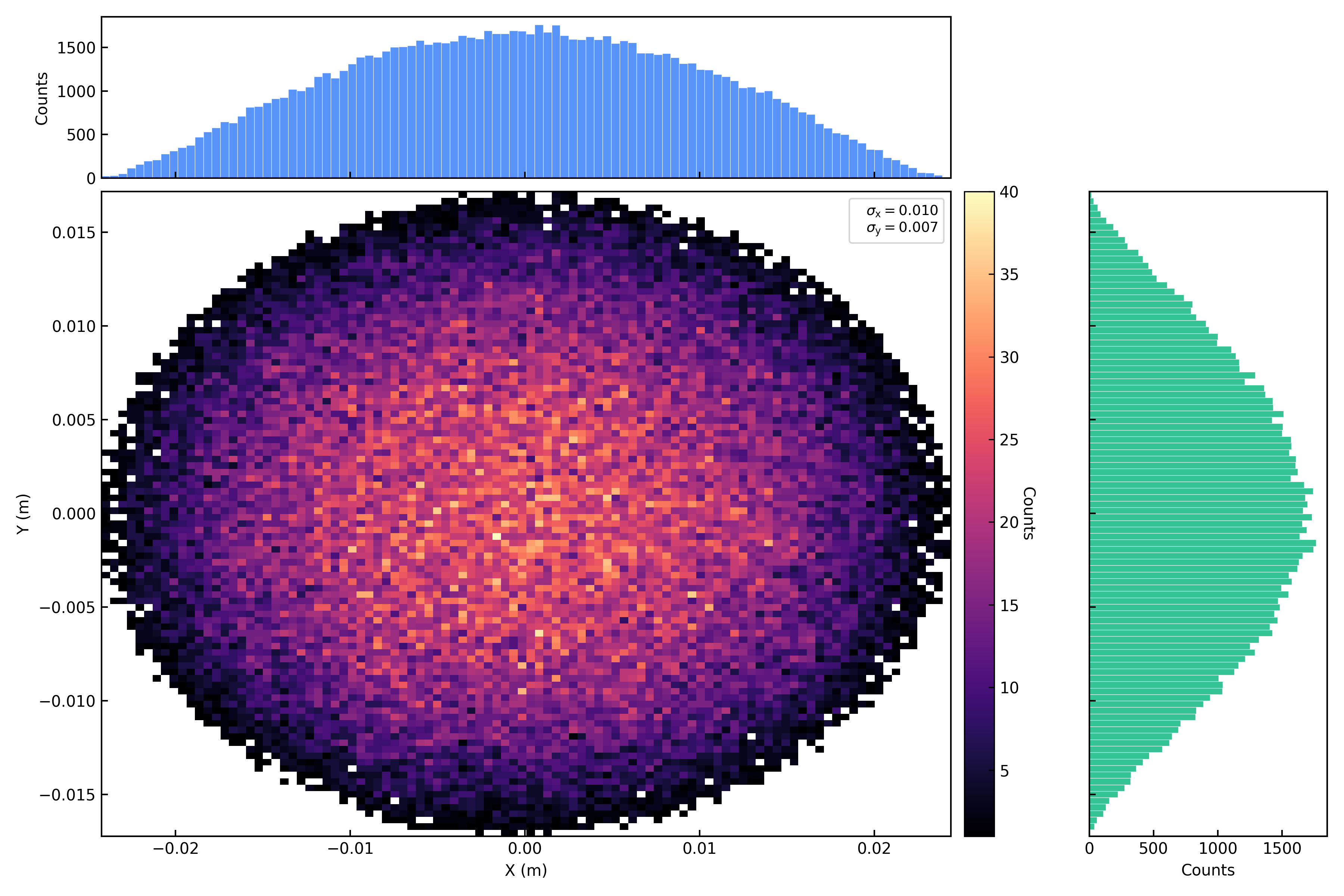
waterbag x-y — Figure 10. Transverse waterbag distribution: x-y

Transverse parabolic distribution:

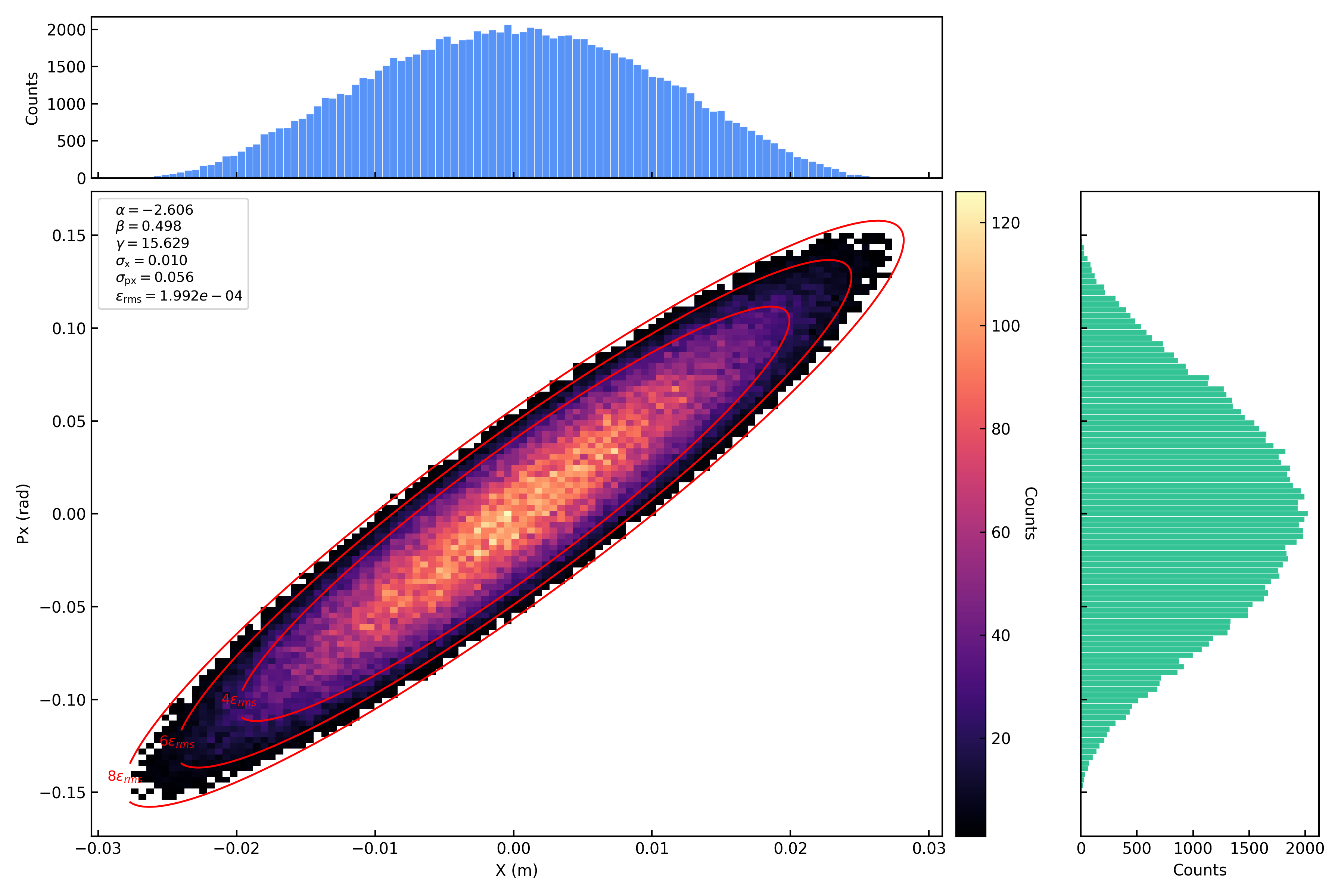
parabolic x-px — Figure 11. Transverse parabolic distribution: x-px

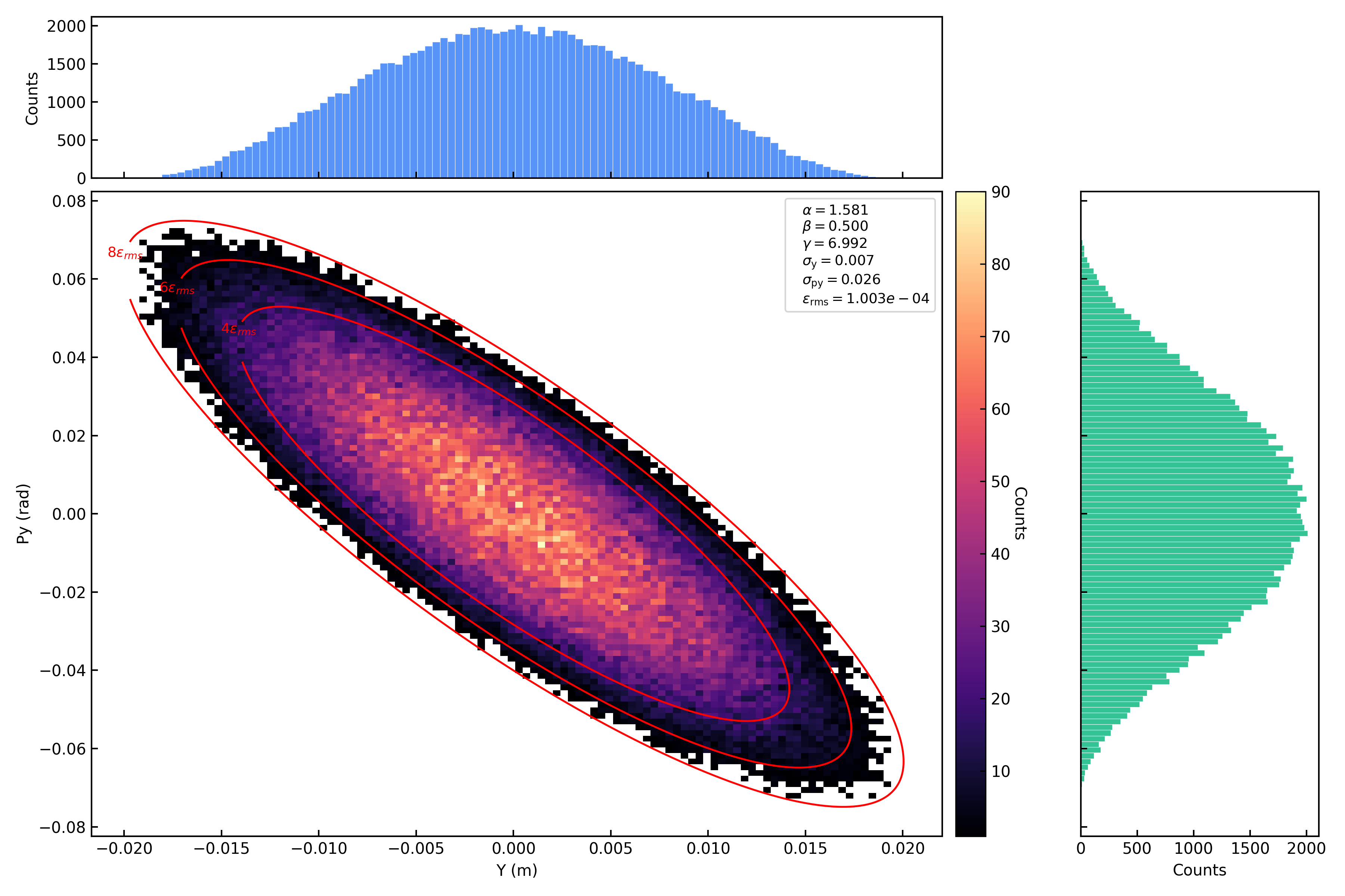
parabolic y-py — Figure 12. Transverse parabolic distribution: y-py

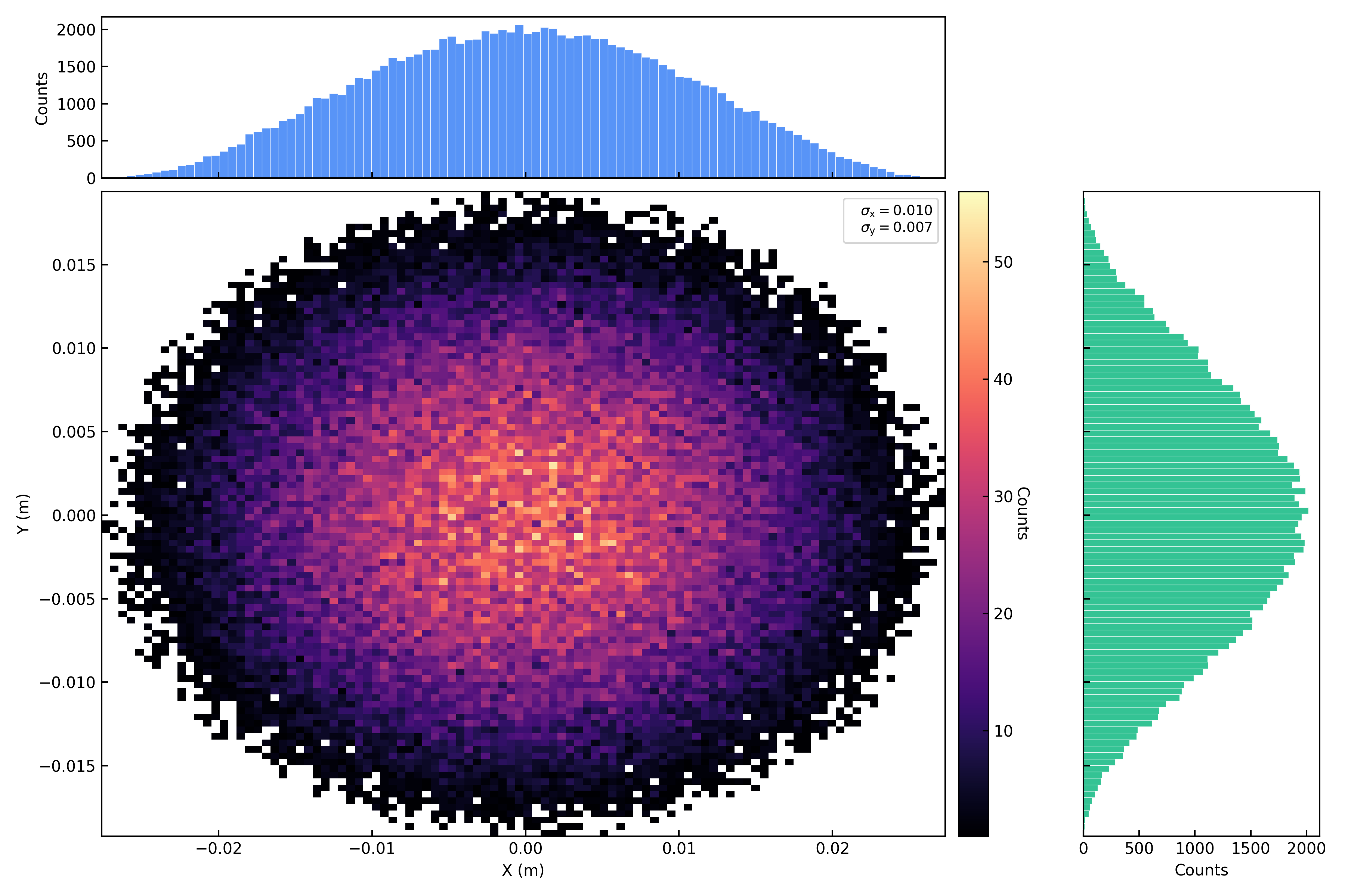
parabolic x-y — Figure 13. Transverse parabolic distribution: x-y

Transverse uniform distribution:

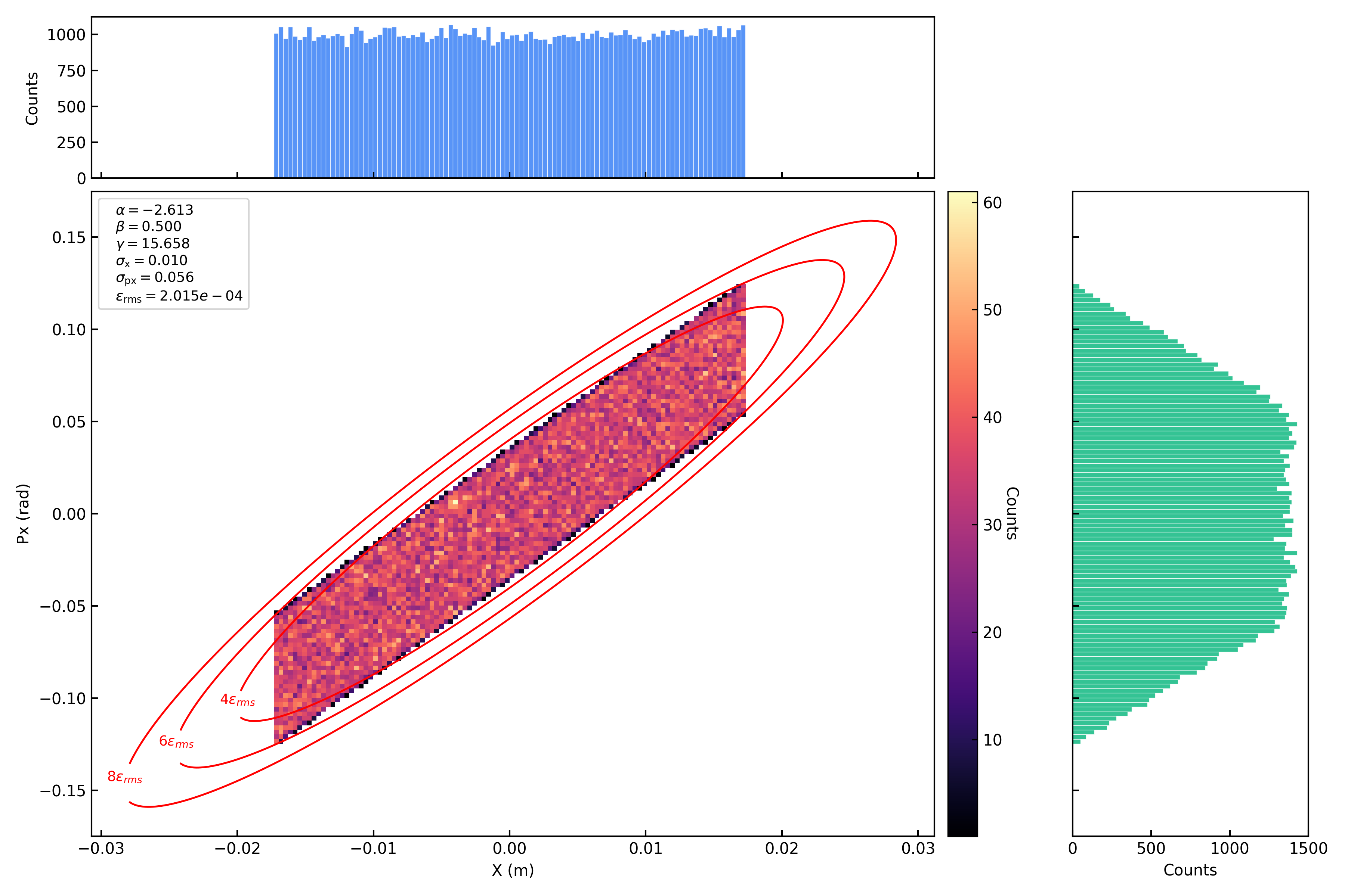
uniform x-px — Figure 14. Transverse uniform distribution: x-px

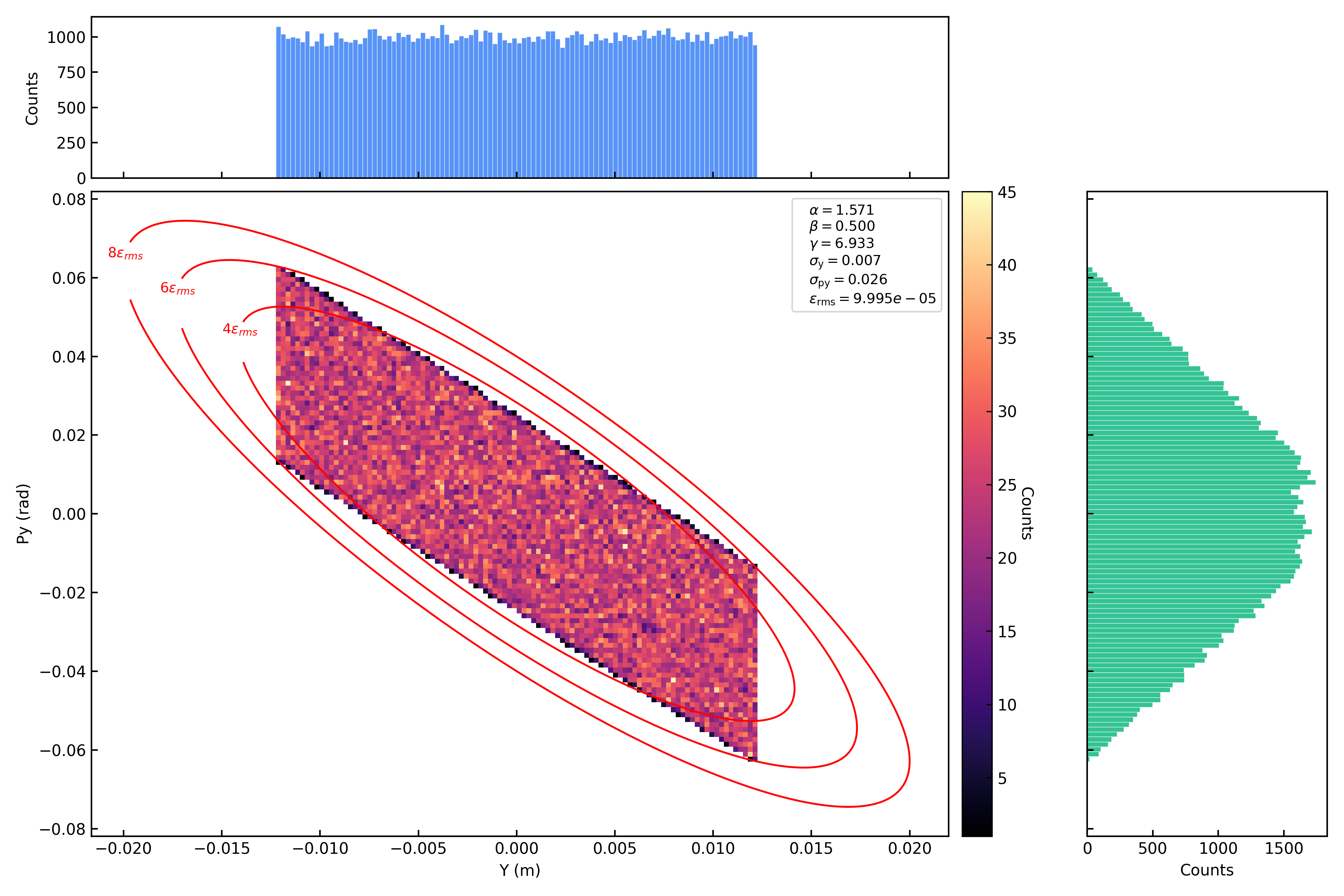
uniform y-py — Figure 15. Transverse uniform distribution: y-py

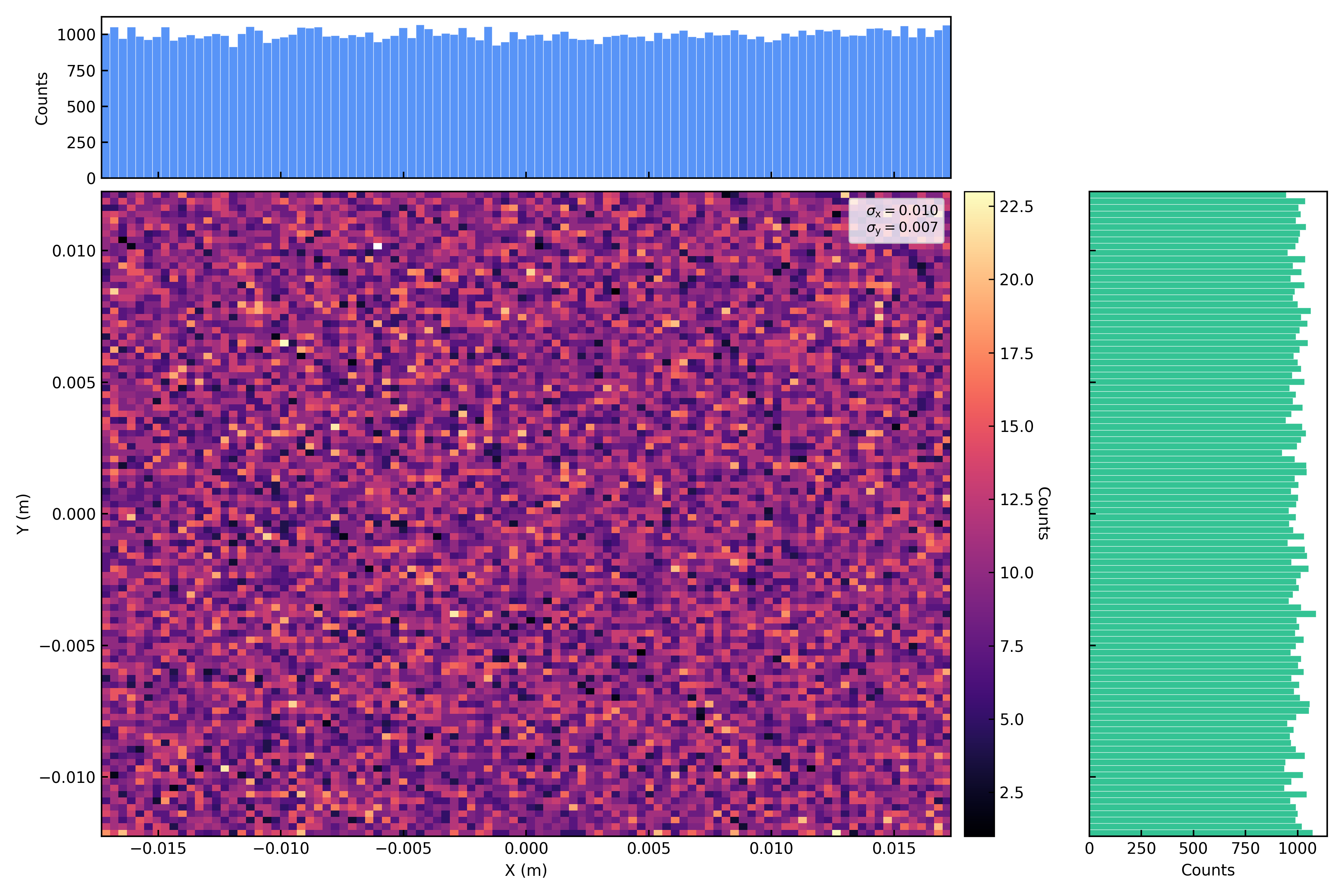
uniform x-y — Figure 16. Transverse uniform distribution: x-y

Longitudinal MatchZ distribution:

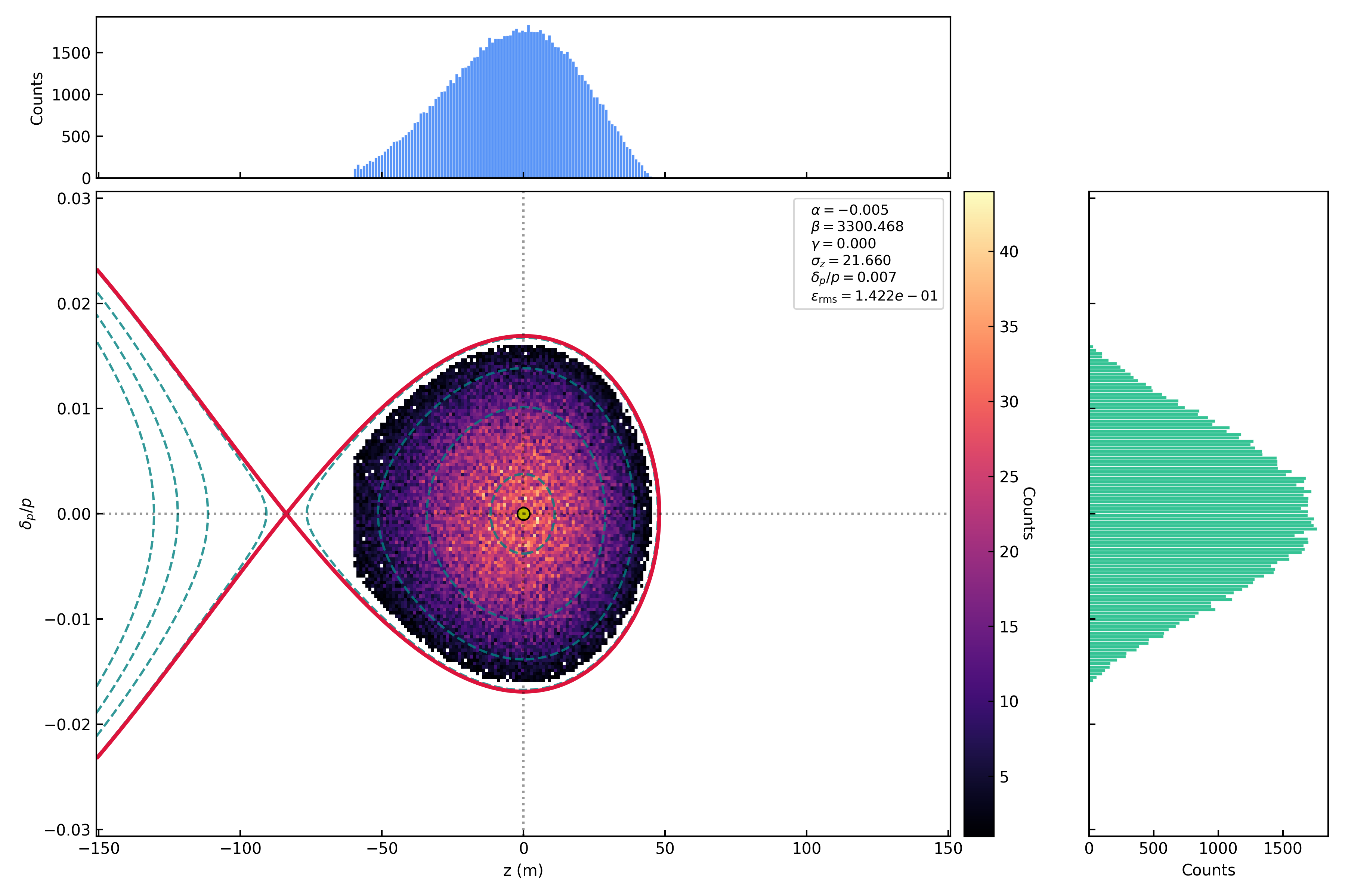
MatchZ z-pz — Figure 17. Longitudinal matchz distribution: z-pz

Longitudinal MatchDp distribution:

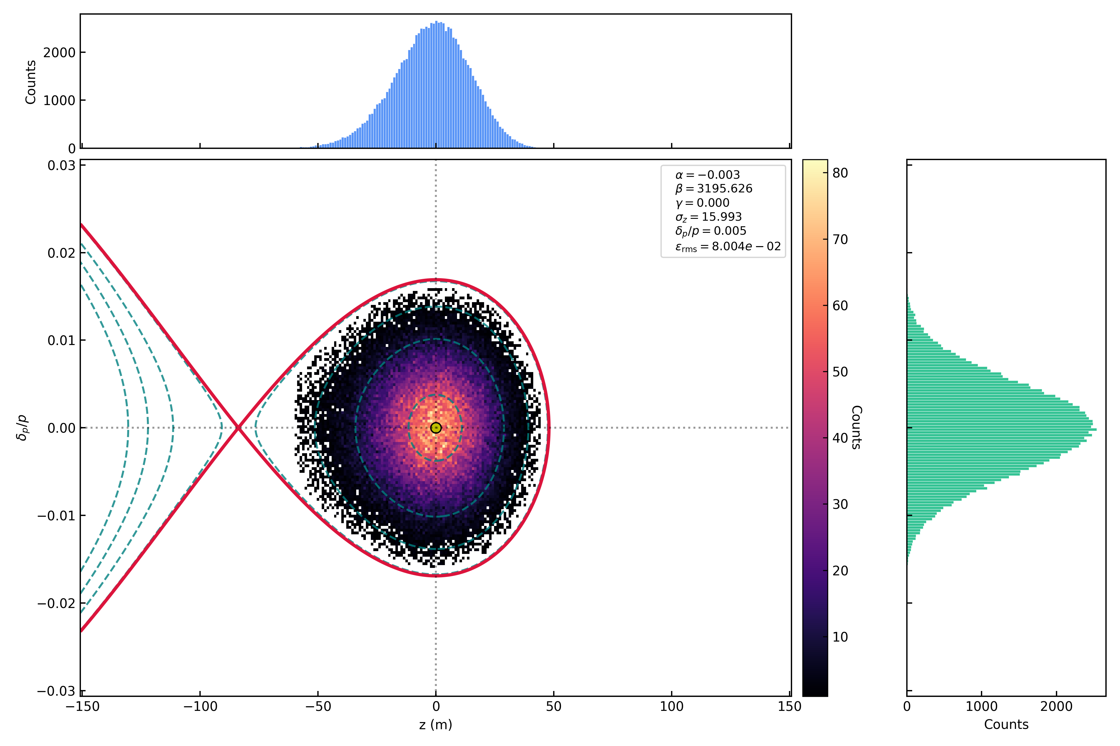
MatchDp z-pz — Figure 18. Longitudinal matchdp distribution: z-pz

Longitudinal Gaussian distribution:

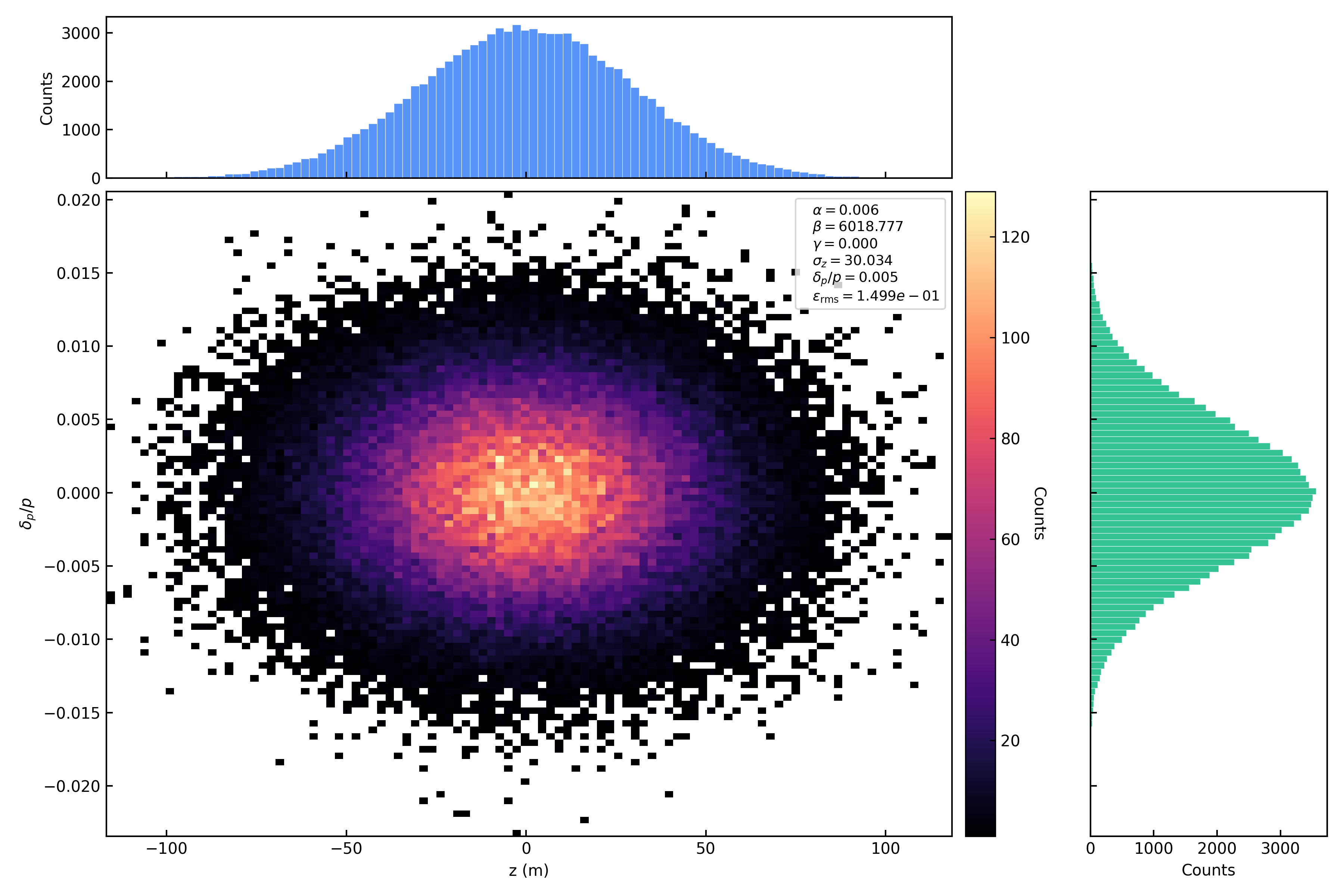
Gaussian z-pz — Figure 19. Longitudinal gaussian distribution: z-pz

Longitudinal Coasting distribution:

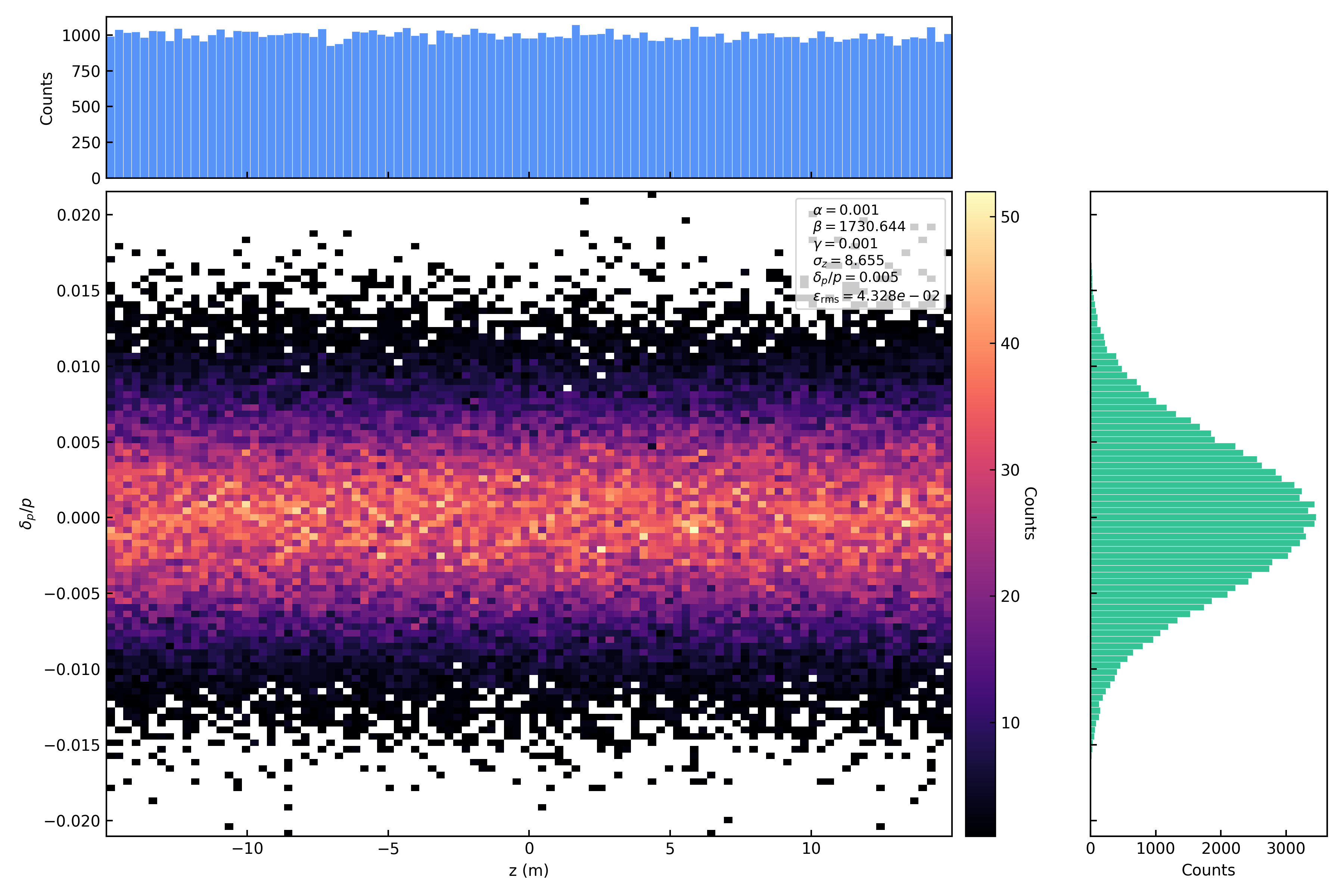
coasting z-pz — Figure 20. Longitudinal coasting distribution: z-pz